This piece is mostly for people who are interested in backtesting
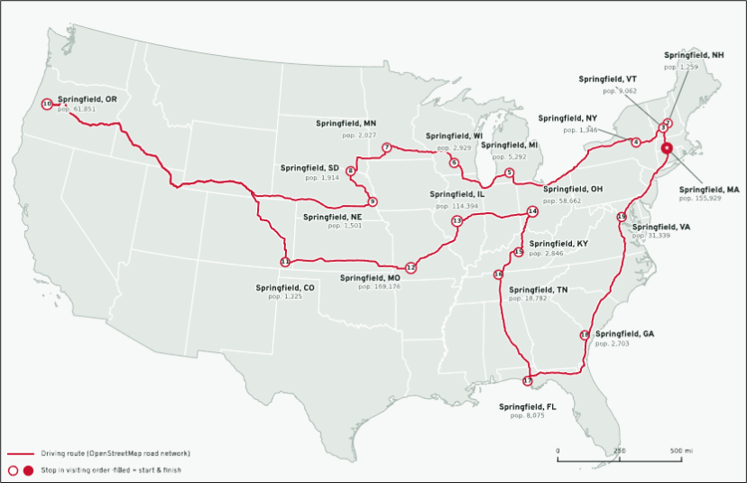
There are 19 Springfields in the United States (minimum population 1,000).
This is the shortest path you can take if you want to drive to all of them.
8,653 miles, 165 hours.
HT CnD

This piece is mostly for people who are interested in backtesting

There are 19 Springfields in the United States (minimum population 1,000).
This is the shortest path you can take if you want to drive to all of them.
8,653 miles, 165 hours.
HT CnD
29OCT 1.1280 EUR call
~30.5 bps off 1.1212 spot
Short 4.95/5.05 USDBRL strangle and buy 4.80/5.20 to protect.
Max gain is what you receive: ~1.65% off 4.98 spot.
Max loss is 1.35% 05NOV expiry
Took off the 4.95 put 16OCT to turn it into a long BRL trade.
Short USDCAD @ 1.4238
Stop loss was 1.4327 now 1.4267
Take profit 1.4011/21 area
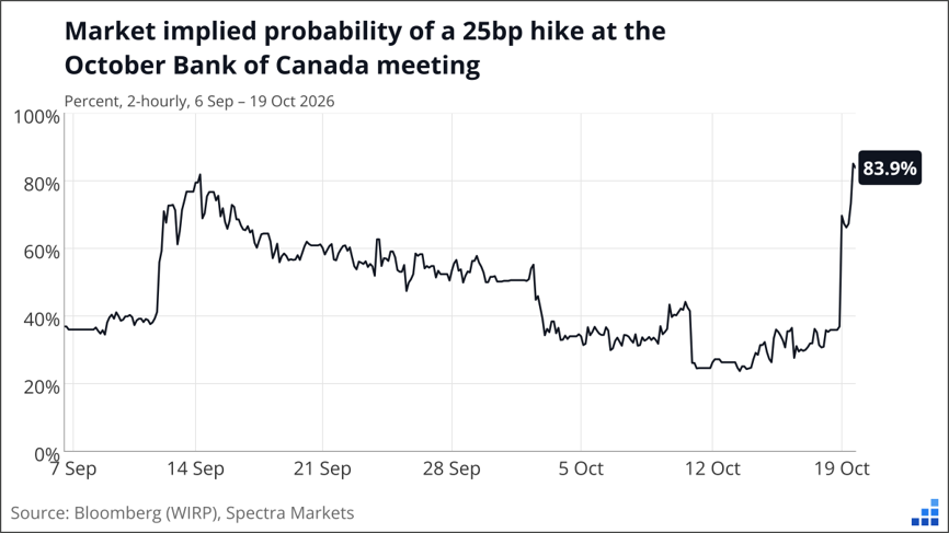
The move in Canadian rates has been fast and furious and another bearish data point for CAD (slightly weaker CPI) has been rejected. Macklem’s weekend statements seem to be paving the way for a rate hike at the end of October, but it’s worth keeping in mind that he doesn’t mind a little surprise here and there. As this hike goes from not really priced to almost fully priced (and the date nears), the risk/reward in USDCAD gets substantially worse. I will be looking to take profit near 1.4000 because I don’t think it’s quite the layup the market is making it out to be.
It’s funny because the market was priced for less than 50% chance of a hike and only 2 out of 23 economists were calling for a hike. But after Macklem’s weekend commentary, BMO, National Bank, and Laurentian all moved to a hike yesterday and the pricing did this:
Bank strategists are sometimes forced into nowcasting instead of forecasting when central bankers signal something and the risk of looking stupid becomes too big to ignore. It’s an odd setup for the Bank of Canada with headline above forecast and core below. This is not unlike the situation in the U.S. where some measures of inflation are hot (CPI and PPI) while trimmed measures are not.
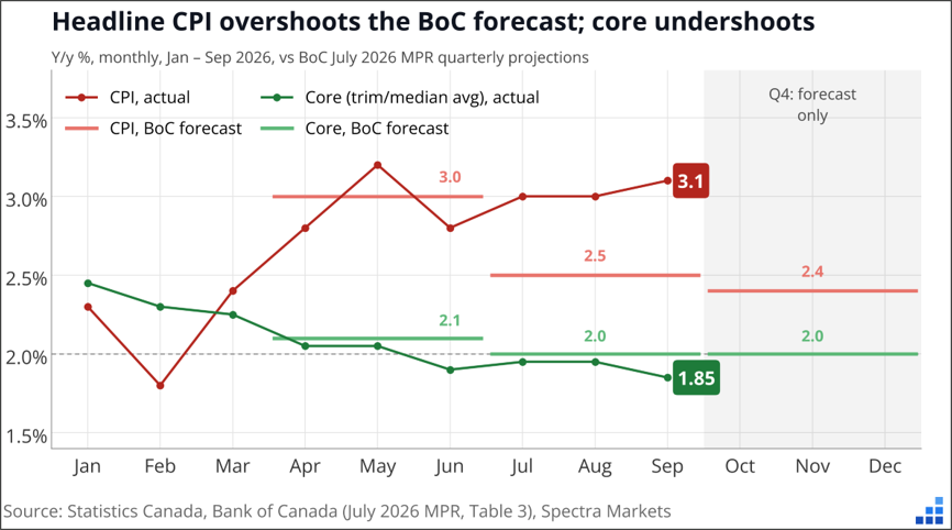
While we are no longer in secular stagnation and thus comparisons to that period are fraught with danger—note that the three other times we had a big headline vs. core divergence like this in Canada (2011, 2018, 2020) headline collapsed back towards core. I suspect this time could be different.
As mentioned, I fear the market is getting a bit too hawked-up here in CAD and that provides a potential opportunity to take some profit. I will cover my USDCAD short between 1.4011 and 1.4021 and be happy. I was only risking 90 pips, so a 220-pip profit is perfectly reasonable.
12-minute read – feel free to forward this piece
A reader and ex-colleague of mine sent me something last week that piqued my interest so I decided to have a peek. He mentioned that a few veteran traders he knows watch a particular planetary setup, Mercury in retrograde, and he looked at what happens when Mercury and Venus are retrograde at the same time. That doesn’t happen very often and when it does, it only lasts a few weeks. And during those periods, the stock market performs extremely (extremely) badly.
With Mercury and Venus in retrograde from October 24 to November 13, I figured I would have a look. Sure, it sounds a bit outlandish, but humans are not rational and I believe there’s more to the world than science can explain. Markets are full of stuff nobody fully understands. And there is documented evidence that mood changes can influence stock market returns. See here, here, and here, for example.
My friend said in his email that since 1975, SPX has returned minus 21% annualized during the Mercury/Venus overlap windows versus +9.5% the rest of the time. Since 2000, the Mercury/Venus window returned minus 65% annualized!! As regular readers know, bearish backtests that actually work on SPX are hard to find because SPX mostly goes up. So, I ran the backtest myself and got the same numbers. It works on Nasdaq too.
Here’s the cleanest way to see it. Split SPX into two buckets: days when Mercury and Venus are both retrograde (I will call this MVR from now on), and all other days. Then, I tried different start dates to see if it stayed robust.
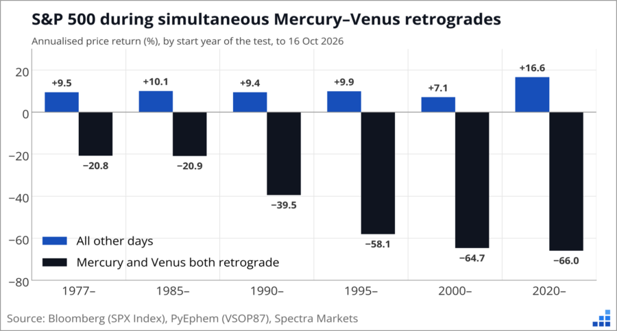
However you slice it, the MVR days lose a lot of money and the rest of the days make money. If you start in 1975, it’s minus 21% annualized during MVR and plus 9.5% the rest of the time. If you start in 1995, it’s −58.1% vs +9.9%. etc.
The signal gets stronger as you move to the more recent data, which could be encouraging. Here’s every one of the windows since 1975, one bar each, with the averages split out on the right. This avoids annualizing, which can sometimes be a trick to make small numbers appear larger.
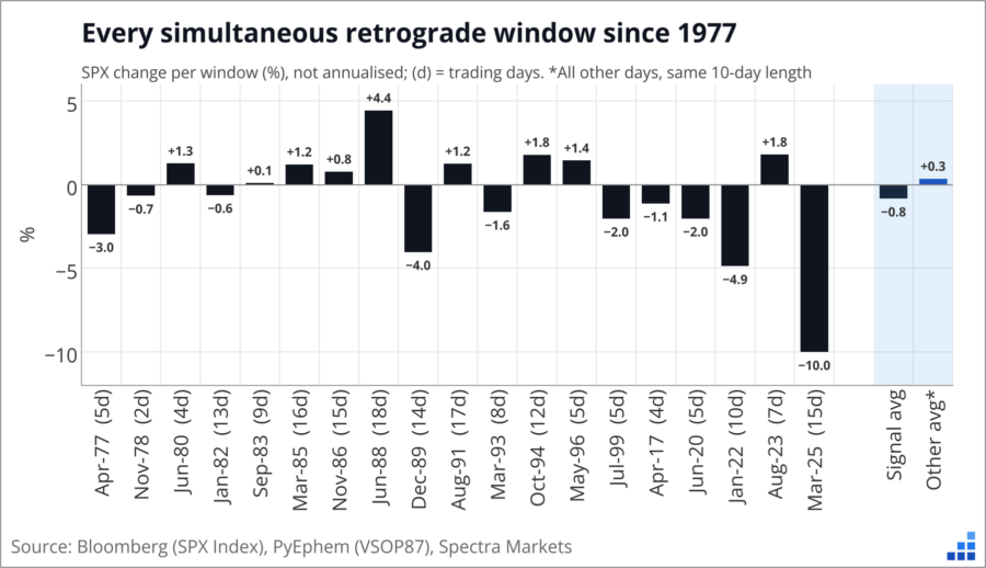
The average window lost 0.8%. A normal 10-day stretch outside the windows gained 0.3%. And just to reiterate—it’s rare to find bearish windows like this in a series like the S&P 500 that has gone up a zillion percent. And this is not just one lucky year. The overlap windows caught the start of the 2022 bear market in January and the Liberation Day crash in April 2025. Since 2000, SPX fell in four of the five windows. Exciting stuff. But like, why would this be a thing? I Googled the astrology, and some of the MVR features are, like:
Mercury and Venus are “inferior” planets that orbit between Earth and the Sun. When they appear to move backward in the sky (an optical illusion caused by Earth passing or being passed in orbit), their retrogrades bring distinct themes of introspection, review, and recalibration.
Introspection, review, and recalibration could be code words for bearish re-evaluation of overheated markets, maybe. But is it real? When there is not a super logical explanation for a sexy backtest like this, I need to keep digging. I always prefer effects like month-end USD moves, where you can explain the movement logically because you know the persistent flow pattern that drives it. Here, the causality (MVR impacts human mood?) is not very clear so I need to keep questioning the data.
Next, I created a trading strategy where you own SPX all the time, but flip short whenever Mercury and Venus are both retrograde. The short covers 184 trading days since 1975, about 1.4% of the time. $100 in buy-and-hold in January 1975 is worth $11,151 today (price only, no dividends). The MVR strategy turns it into $15,314, or 10.2% a year vs 9.5%. But when you chart it, it’s not as exciting as the data makes it sound. Charting a strategy can often reveal undesirable features of that strategy.
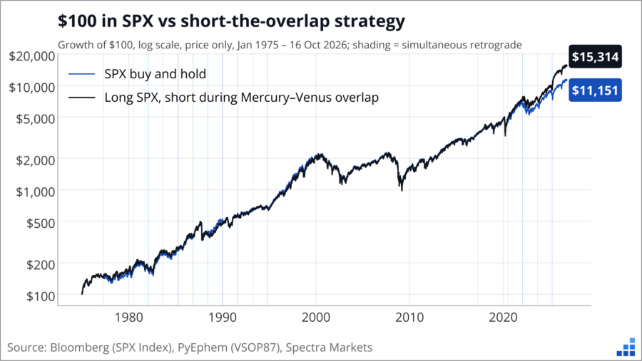
Hmm, look at the chart. The two lines track each other for 25 years. All the outperformance comes after 2020.
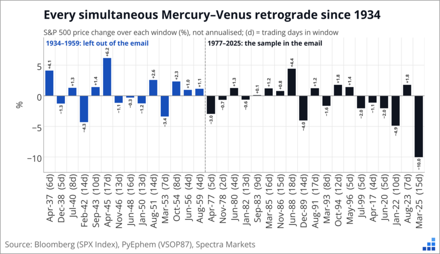
Next, I added back the history the initial backtest left out. Our SPX data goes back to 1928, so here are the same windows going all the way back to 1934. This is a quick way to get some out of sample data to compare to the 1975 to now sample we used before. A quick eyeball suggests the out of sample results are not as impressive.
Here’s the catch: Mercury and Venus aren’t the only pair astrologers watch. And this is the key here. We have the results of the MVR trade but hidden in plain sight is the fact that there are many, many other planetary combinations that might have been tried before the Mercury + Venus retrograde combo finally worked.
One of the trickiest things in handling data is trying to figure out what data you are not seeing. What is the missing data that might be influencing the result? Here’s an excerpt from Alpha Trader that explains the concept of missing data and why and how it’s so nefarious and tricky.
Survivors and incomplete samples
People don’t always think about whether their sample is complete or biased
In World War 2, the US Navy wanted to reduce the number of its fighter planes being shot down and wanted to add armor at various points to reinforce the fighters. Armor increases a plane’s weight and makes it less efficient, so you need to be selective about where to put armor. The statisticians in the wartime Statistical Research Group received a diagram showing data something like this:
Distribution of bullet holes in damaged US fighter planes
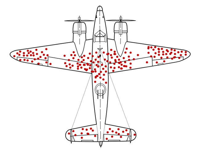
The intuitive or obvious answer is to reinforce the areas that are getting hit by enemy fire. The wings, fuselage, and tail look like natural places to add armor since they get shot up the most.
But legendary mathematician Abraham Wald ignored the intuitive answer and thought more deeply. He thought to ask: “Why are there so many holes in the fuselage and wings, but no bullet holes in the engines?”
This is like asking: why are there so many ER patients with gunshot wounds to the arm but so few with gunshot wounds to the heart, even though both sections of the human body are in a similar area? The answer, of course, is that the planes that got shot in the engine went down and were destroyed, so they couldn’t be examined. There are no bullet holes in the engines of the planes that return to base because the planes that are shot in the engine don’t make it back to base. Victims shot in the heart don’t make it to the ER.
Survivorship bias is the phenomenon where we evaluate a sample (say planes returning from battle or mutual funds) and then draw conclusions based on that sample without considering all the parts of the sample that did not survive. We look at planes that returned to base without considering the ones that got shot down. We look at performance of existing mutual funds without considering all the ones that went out of business. This is another way we misinterpret data.
Here’s one way this applies to trading. A friend of yours shows you a specific strategy that earned 1105% returns last month. Your first reaction might be “Wow, tell me more!” When really your first reaction should be: “What other strategies did you test before coming up with this one?”
When analyzing data, look for missing evidence.
This is a common trick in the sports gambling industry. Say the Tigers are playing the Bears tonight. You send 10,000 e-mails out to new prospects. 5,000 of the e-mails read: “Attention subscribers: OUR GOLD STAR, GUARANTEED PICK TONIGHT IS: TIGERS TO WIN!” and 5000 say: “Attention subscribers: OUR GOLD STAR, GUARANTEED PICK TONIGHT IS: BEARS TO WIN!” Then, they wait to see who wins. Let’s say it’s the Tigers.
The next game is Lions vs. Panthers. The marketer now takes the list of 5,000 e-mails that received the correct Tigers pick e-mail and splits those into two groups of 2,500. Half the e-mails predict the Lions and half predict the Panthers. They do this twice more and now have a list of 625 people that just received FOUR STRAIGHT GOLD STAR PICK WINNERS! Then, they call up those 625 prospects (many of whom are suitably impressed—nobody else had the Panthers to beat the Lions in that game!) and try to close the deal on a $1,200/year subscription to the GOLD STAR PICK SHEET.
Those bettors that got the four accurate e-mails in a row have to be very smart to think of the hidden evidence they might be missing. More likely, their emotional desire to win overrides their logical or rational mind and they hand their credit card number over to the waiting operator.
End of excerpt from Alpha Trader
So going back to our story here, there are 7 planets that can be in retrograde, plus 21 different ways that two planets in our solar system could be in retrograde at the same time. We are talking about Mercury and Venus, but what if we test Mars and Saturn, for example? And Mercury on its own? Jupiter and Neptune? Etc.
Sorry Pluto, you don’t count, loser.
Now you have 28 backtests to run. I tested them all on SPX back to 1975. Venus and Mars were never retrograde together in that time, so that’s 27 setups to test. The strongest is our MVR (Mercury and Venus), with a t-stat of −1.58. Ideally you want a t-stat of two or more to get excited. With 27 tries, you’d expect one or two tests to clear two by pure chance. Zero did.
So that’s data mining in a nutshell. Test enough things and one of them will look amazing. To measure how much luck to expect, I ran a shuffle test. I slid the whole planetary calendar forward by a random amount, so the planets keep their real rhythms but lose any link to real dates. Then I reran all 27 setups, 1,000 times.
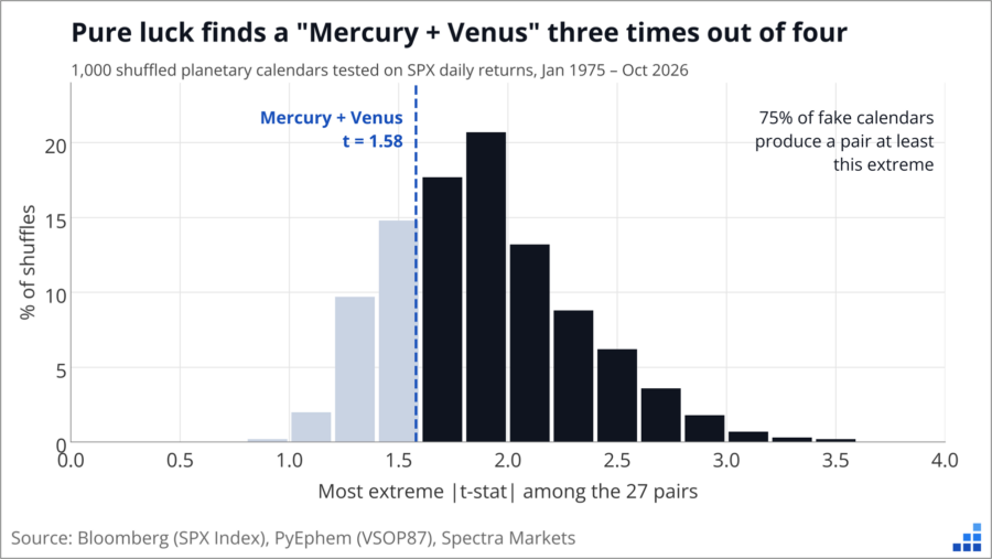
In 75% of the fake calendars, at least one pair looked as extreme as Mercury + Venus. Random dates pull this off three times out of four. That tells you how much of the original result could be luck.
This is called the garden of forking paths. When you start a backtest, you walk through a series of decisions. A series of forks in the path, as it were. Should I pick Mercury alone, or a pair? SPX, Nasdaq or the Nikkei? Annualized or raw data? Start in 1965, 1975 or 2000? The email from my reader starts in 1975, which ignores 14 windows from 1934 to 1959. Those were net positive. Each choice down the forking path looks harmless, but when you keep adding them together, you are more likely to find pyrite, not gold.
If you are not familiar with the concept, here’s a short garden of forking paths explainer:
The garden of forking paths is a statistical problem in which researchers make a series of seemingly reasonable decisions about how to analyze data—what variables to include, which time periods to examine, how to handle outliers, and which relationships to test—but those decisions are influenced, consciously or unconsciously, by the results they see along the way.
Even without deliberately cherry-picking results, researchers can end up with statistically significant findings that are largely products of chance, because countless alternative analytical paths were available. The concept was popularized by statisticians Andrew Gelman and Eric Loken in a 2013 paper, The Garden of Forking Paths, and takes its name from Jorge Luis Borges’s 1941 short story The Garden of Forking Paths, which explores the idea of multiple branching realities.
In financial backtesting, the problem is especially dangerous: a trader can test different indicators, lookback periods, entry rules, and stop-loss levels until a compelling historical Sharpe ratio emerges, without realizing that the apparent edge may simply be the lucky survivor of hundreds of possible strategies. The crucial insight is that you don’t have to consciously data-mine to produce a data-mined result.
The best way to check for luck is to test data nobody looked at when the pattern was found (i.e., out of sample data). Our SPX history runs back to 1928, so I took the two standout pairs (MVR and the most bullish pair, Venus plus Saturn) and checked the out of sample data.
Mercury + Venus was 12.8bp a day worse than other days from 1975 onward. Before 1975 it was 3.7bp a day better. Venus + Saturn was 9.9bp a day better from 1975. Before 1975 the edge was 1.4bp, with a t-stat of 0.19. It’s noise.
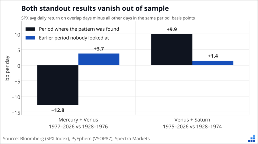
When you test a bunch of stuff, the most extreme results are the most likely to be flukes, and flukes shrink back toward average when you give them new data. Both of these shrank. When you are presented with a backtest, one of the most important questions you need to ask is: What data was omitted from this test? In this case, lots of data! Especially the fact that there are 27 planet and retrograde setups that one might test if one were looking for cool or spooky Halloween bear treats!
To show how easy it is to manufacture a signal like this, I split every SPX day since 1928 by moon phase (8 phases), day of the week (5) and month (12). That’s 480 combinations. Then I searched 1928 to 1999 for the best time to be long stocks. The winner: Thursdays in July when the moon is waning gibbous. From 1928 to 1999, SPX averaged +39bp on those days. That’s 16 times a normal day, with a t-stat of 3.67.
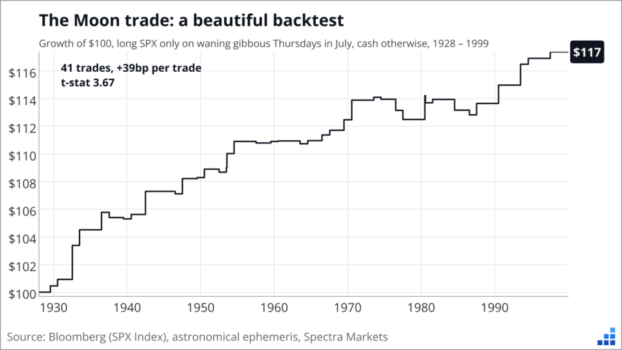
Peer review that, suckah!
Then I ran it on 2000 to 2026, the out of sample bit.
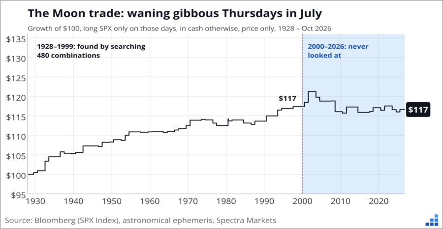
$100 grows to $117 by 1999. It’s still $117 today. The 17 trades since 2000 averaged −3.8bp.
The first principle is that you must not fool yourself—
and you are the easiest person to fool
– Richard Feynman
None of this is specific to astrology. Switch “Mercury is in retrograde” for “the third Friday after an FOMC” or “when the VIX term structure inverts” and the same traps often apply. Before you trust a backtest, think about the following:
Big thanks to the reader who sent this in. It’s a good example of how backtests can be super convincing. My gut reaction initially was not skepticism, it was: WHOA! This scenario has many of the spiciest ingredients you need to make a backtest look better than it is: a small sample, annualized returns, driven by two crashes, found inside a big search, with an inconvenient chunk of history left out.
That doesn’t mean the idea is silly. Science doesn’t know everything! I’m just saying this particular dataset can’t tell a real effect from luck. The next simultaneous window for Mercury and Venus in retrograde runs from 24OCT to 13NOV, about 15 trading days right through Halloween. If SPX falls, I guess you were warned?
:]
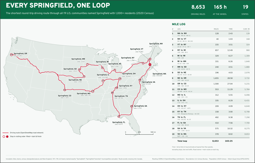
There are 19 Springfields in the United States (minimum population 1,000, using 2020 census data).
This is the shortest path you can take to drive to all of them.
8,653 miles, 165 hours of driving.
Calculating this optimal path is fiendishly complicated and is known as the Traveling Salesman Problem.
The Traveling Salesman Problem is one of the most famous problems in mathematics and computer science. It’s classified as NP-hard, meaning there is no known algorithm that solves every instance efficiently as the number of places grows. In this instance, I used the Held-Karp method, which uses dynamic programming instead of checking every route individually. There are 3.2 quadrillion (that is 18!/2) distinct ways of starting somewhere, visiting each of the 19 places exactly once, and returning to the start.
Calculating the routes one-by-one would not have been very fun.
HT CnD